Why Stacking Sliding Windows Can't See Very Far

Modern language models like GPT-OSS, Mistral, Llama-4, and Gemma 3 use a building block called sliding window attention (SWA) to handle long texts efficiently. Instead of letting each word look at all previous words (which becomes computationally expensive), SWA restricts each word to only "see" the last $W$ words—similar to reading through a sliding window.

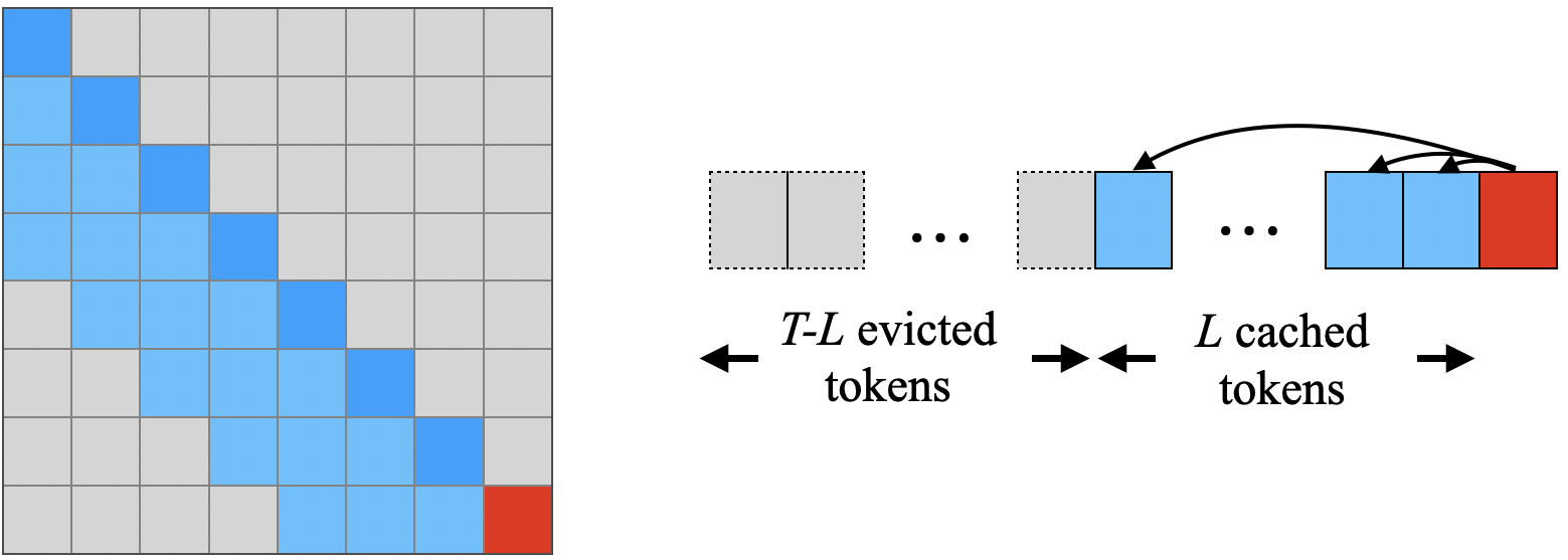
Sliding window attention illustration from the StreamingLLM paper. Each token can only attend to a constant number of previous tokens, dramatically reducing computational complexity while maintaining local context.

Here's the puzzle: if you stack $L$ layers of sliding window attention, shouldn't the model be able to see $L \times W$ words back? After all, in this idealized scenario where each layer only performs sliding window attention (without any other mechanisms), information can hop backward exactly $W$ positions at each layer. With 100 layers and a window of 1,000 words, that's theoretically 100,000 words of context!

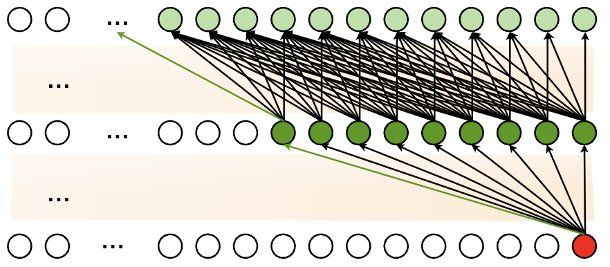
Theoretical information propagation in sliding window attention from the PowerAttention paper. Information can theoretically hop backward $W$ positions at each layer, creating a receptive field that grows linearly with depth. However, this idealized view doesn't account for information dilution and residual connection effects.

However, in practice, SWA models struggle to use information from more than about 1,500 words ago—far less than the theoretical 100,000. What explains this significant gap?

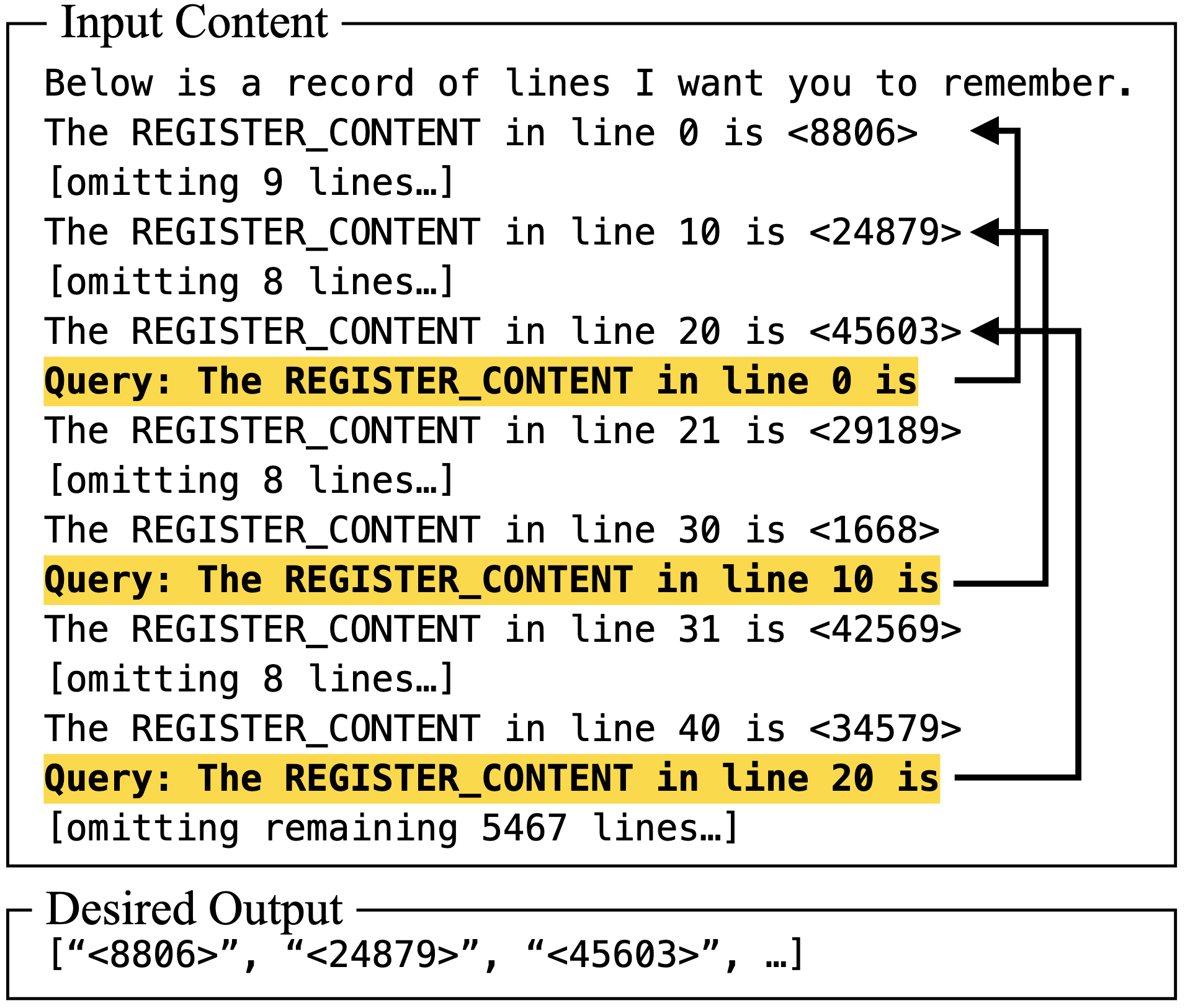
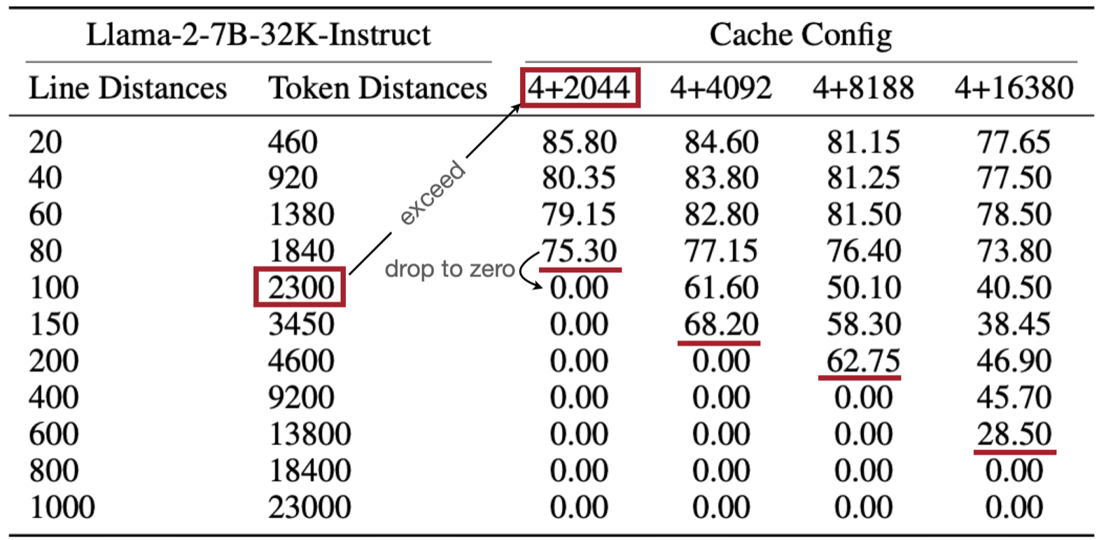
Empirical evidence of the gap between theory and practice. Left: Task formulation from the StreamingLLM paper, where the model must answer about a specific number that appears several lines before in the context. Right: Performance results showing that StreamingLLM's (can be seen as a pure SWA model) accuracy drastically drops once the queried information is no longer in the sliding window cache, despite the fact that this information should theoretically be propagated through the network layers.

In this post, I'll build a mathematical model that explains this discrepancy. The answer involves two key effects that limit how far back these models can effectively access information:

Information gets diluted as it spreads through the network (like a game of telephone)
Residual connections create an exponential barrier that blocks distant information

Let's explore why the effective memory of these models has fundamental limitations, regardless of their depth.

What is Sliding Window Attention?

In standard attention, each position can look at all previous positions—like having access to the entire preceding context. The computation is:

\text{Attention}(Q, K, V) = \text{softmax}\left(\frac{QK^T}{\sqrt{d_k}}\right)V

With sliding window attention, each position can only see the last $W$ positions:

\text{SWA}(Q, K, V)_t = \text{softmax}\left(\frac{Q_t K_{[t-W+1:t]}^T}{\sqrt{d_k}}\right)V_{[t-W+1:t]}

For example: when processing token 1000, the SWA layer can only directly see tokens 901-1000 (if $W=100$). This reduces computation from $O(n^2)$ to $O(nW)$—making it more tractable for long texts.

Part I: Tracking Information Flow Through Layers

How Does Information Travel?

To understand this problem, we need to track how information flows through the network. We want to quantify how much influence a word at position $i$ has on the computation at position $t$ after going through $l$ layers.

Let's call this influence $P_l(d)$, where $d = t - i$ is the distance between the positions. For example:

$P_l(0)$ = influence of the current position on itself
$P_l(10)$ = influence of a word 10 positions back
$P_l(100)$ = influence of a word 100 positions back

These influences must sum to 1 (since the total contribution from all positions equals 100%).

A Simplifying Assumption

To make the math tractable, I'll assume that on average, attention weights are uniformly distributed across the window. In other words, each of the $W$ visible positions gets equal attention:

\text{Average attention to each position} = \frac{1}{W}

This isn't exactly true for trained models (they learn to focus on important words), but it captures the fundamental architectural bias—the starting point that any learned pattern must work from. This uniform assumption allows us to analyze the architectural bias before any learning has occurred. A trained model will learn non-uniform attention patterns, but it must do so on top of this underlying architectural prior. Therefore, the limits we derive represent a fundamental baseline the model must overcome.

Let's start with the simpler case: what happens without residual connections?

Case 1: Pure SWA (No Residual Connections)

Interactive Visualization: Explore how information flows through stacked sliding window attention layers without residual connections. The distribution evolves from a uniform window (L=1) to a Gaussian-like spread (L>3) due to repeated convolution. Notice how the effective range grows as √L, not linearly with depth.

Let's first imagine a simplified world where each layer just does sliding window attention, nothing else:

h_t^{(l)} = \text{SWA}(h^{(l-1)})_t

In this case, each position averages information from the $W$ positions in its window.

What Happens at Each Layer?

Layer 1: The influence distribution is uniform across the window. If $W=100$, then each of the last 100 positions contributes $\frac{1}{100}$ to the output. Positions beyond the window contribute nothing:

P_1(d) = \begin{cases} \frac{1}{W} & \text{if } d < W \\ 0 & \text{if } d \geq W \end{cases}

Layer 2 and Beyond: For a distant token to influence the current position, it needs to propagate through intermediate positions:

The distant token influences some intermediate position at layer 1
That intermediate position then influences the current position at layer 2

Mathematically, the influence at layer $l$ becomes a convolution:

P_l(d) = \sum_{j=0}^{W-1} P_{l-1}(d-j) \cdot \frac{1}{W}

This says: to influence position $t$ from distance $d$, information can first travel to any intermediate position (distance $d-j$), then hop the remaining $j$ positions.

The Central Limit Theorem Kicks In

After many layers of this convolution process, the influence distribution $P_L(d)$ will spread out and can be approximated by a Gaussian (bell curve) due to the central limit-like behavior of repeated convolution. To see why, let's track the statistics.

At each layer, we "look back" a random distance uniformly distributed over $[0, W-1]$. Think of the total distance $d$ that information travels after $L$ layers as the sum of $L$ independent 'hops', where each hop's distance is a random variable drawn uniformly from $\{0, 1, ..., W-1\}$. The Central Limit Theorem tells us that the distribution of this sum will approach a Gaussian.

Galton Board: Just like balls falling through pegs create a bell curve, information "hopping" through layers creates a Gaussian distribution of influence. Each layer adds randomness, and the sum of many random hops naturally forms the familiar bell shape.

The mean and variance of a single hop are:

\mu_1 = \frac{1}{W}\sum_{j=0}^{W-1} j = \frac{W-1}{2}

\sigma_1^2 = \frac{1}{W}\sum_{j=0}^{W-1} j^2 - \mu_1^2 = \frac{(W-1)(2W-1)}{6} - \left(\frac{W-1}{2}\right)^2 = \frac{W^2-1}{12}

After $L$ layers, by the central limit-like behavior of repeated convolution:

Mean total lookback: $\mu_L = L \cdot \mu_1 = \frac{L(W-1)}{2} \approx \frac{LW}{2}$
Variance: $\sigma_L^2 = L \cdot \sigma_1^2 = \frac{L(W^2-1)}{12}$
Standard deviation: $\sigma_L = \sqrt{\frac{L(W^2-1)}{12}} \approx 0.29W\sqrt{L}$

The Result: $O(W\sqrt{L})$ Growth

The effective receptive field—how far the model can meaningfully see—is determined by the width of this bell curve:

$$\text{Effective Range} \approx W\sqrt{L} \text{ (not } LW\text{!)}$$

This is an important finding: even without residual connections, the effective range grows only as the square root of depth, not linearly. This $\sqrt{L}$ scaling relationship was also characterized in the context of convolutional neural networks by Luo et al. (2017), who showed that effective receptive fields follow Gaussian distributions and grow sublinearly with network depth.

Why? Information dilution. As information spreads through layers, it gets averaged and re-averaged, dispersing across many positions. After 10 layers, information from any single distant token is highly diluted.

Example: With $W=100$ and $L=100$ layers:

Theoretical receptive field: $100 \times 100 = 10,000$ tokens
Effective receptive field: $100 \times \sqrt{100} = 1,000$ tokens

That's already a 10× reduction. The situation becomes even more constrained when we add residual connections.

Part II: The Impact of Residual Connections

What Are Residual Connections?

Modern transformers don't just pass information through attention layers. They use residual connections (also called skip connections) that let most information bypass each layer unchanged:

h_t^{(l)} = h_t^{(l-1)} + \text{Attention}(h^{(l-1)})_t

Transformer architecture showing residual connections

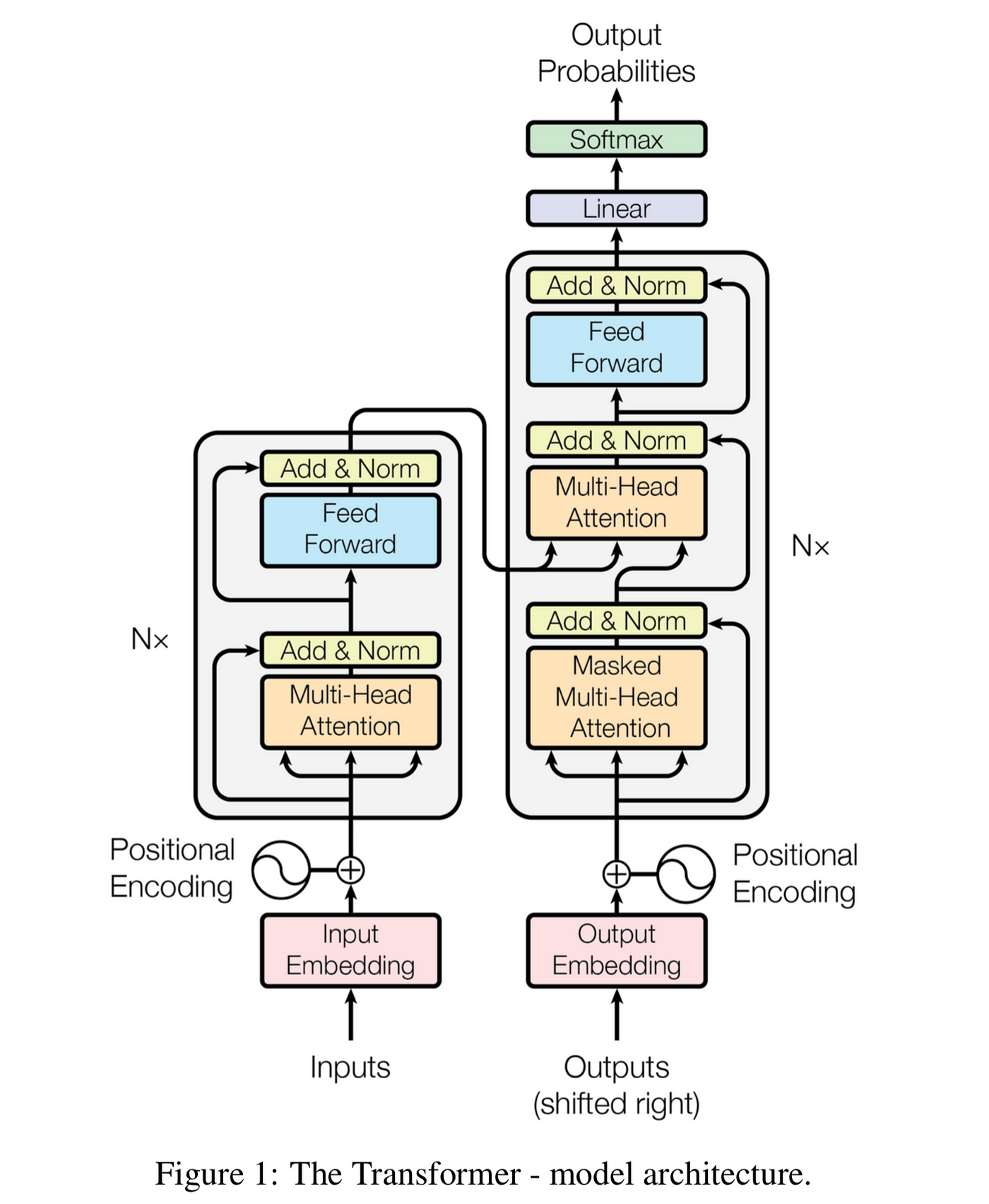
The Transformer Architecture: The "Add & Norm" components implement residual connections, allowing information to bypass each layer. This architectural choice fundamentally shapes how information flows through the network. (Figure from Attention Is All You Need)

We can model this behavior as a weighted average:

h_t^{(l)} = \alpha \cdot h_t^{(l-1)} + (1-\alpha) \cdot \text{SWA}(h^{(l-1)})_t

where $\alpha$ represents the conceptual strength of the residual path. In real models, which include LayerNorm, $\alpha$ isn't an explicit parameter but an emergent property of the system, typically very close to 1 (0.9-0.99)—meaning 90-99% of the information effectively bypasses the attention layer.

Two Competing Information Highways

This creates two parallel paths for information:

The Direct Path (weight $\alpha$): Information passes straight through, position to position
The Attention Path (weight $1-\alpha$): Information flows through the attention window

Most information stays on the direct path, while only a small fraction goes through the attention mechanism. This architectural choice has significant consequences.

Case 2: SWA with Residual Connections

Interactive Visualization: Observe the dramatic impact of residual connections on information flow. The "spike-and-slab" pattern shows a massive concentration at the current position with exponentially decaying influence for distant tokens. Try adjusting α to see how stronger residuals create tighter locality bias. The effective horizon remains fixed regardless of layer depth L.

The Spike-and-Slab Pattern

With residual connections, the update equation at each layer becomes:

h_t^{(l)} = \alpha h_t^{(l-1)} + (1-\alpha) \cdot \frac{1}{W} \sum_{j=t-W+1}^{t} h_j^{(l-1)}

This creates a distinctive influence distribution after the first layer:

P_1(d) = \begin{cases} \alpha + \frac{1-\alpha}{W} & \text{if } d=0 \quad \text{(strong peak at current position)} \\ \frac{1-\alpha}{W} & \text{if } d \in [1, W-1] \quad \text{(small uniform background)} \\ 0 & \text{if } d \geq W \end{cases}

This creates a distinctive 'spike-and-slab' distribution, a term borrowed from Bayesian statistics, with a massive 'spike' of influence at the current position and a tiny, flat 'slab' of influence across the rest of the window.

To see why: the current position ($d=0$) gets contribution $\alpha$ from the residual path plus $\frac{1-\alpha}{W}$ from being in the attention window.

Example with numbers: If $\alpha = 0.95$ and $W = 100$:

Current position ($d=0$): $0.95 + \frac{0.05}{100} = 0.9505$ (95.05% of the weight)
Each other position in window: $\frac{0.05}{100} = 0.0005$ (0.05% of the weight)

That's a 1900× difference. The model strongly favors preserving local information.

The Exponential Decay Effect

For subsequent layers, the recurrence relation becomes:

P_l(d) = \alpha P_{l-1}(d) + \frac{1-\alpha}{W} \sum_{j=0}^{W-1} P_{l-1}(d-j)

(where $P_{l-1}(k)=0$ for $k<0$)

This says: influence at distance $d$ comes from either:

The residual path preserving influence already at distance $d$ (weight $\alpha$)
The attention path aggregating influences that can reach $d$ through convolution (weight $1-\alpha$)

Here's the critical insight: for information to travel distance $d > W$, it must take at least $k = \lceil d/W \rceil$ "hops" through attention windows (since each hop bridges at most $W$ positions).

Key observation: Each time information goes through the attention path instead of the residual path, it gets multiplied by $(1-\alpha)$. This suggests that the influence from a distance $d$ will be bounded by an exponential decay:

P_l(d) \leq C \cdot (1-\alpha)^{\lceil d/W \rceil}

In practice, this upper bound behaves like a very good approximation for the actual influence. For large $d$, this can be written as:

P_l(d) \approx C \cdot (1-\alpha)^{d/W} = C \cdot e^{-\lambda d}

where $\lambda = -\ln(1-\alpha)/W$ is the decay rate.

Example: With $\alpha = 0.95$:

After 1 window-width: $(1-0.95)^1 = 0.05$ (5% remains)
After 2 window-widths: $(1-0.95)^2 = 0.0025$ (0.25% remains)
After 3 window-widths: $(1-0.95)^3 = 0.000125$ (0.0125% remains)

This exponential barrier is why depth doesn't help—adding more layers can't overcome exponential decay.

Part III: The Effective Horizon Formula

How Far Can Models Really See?

Let's quantify exactly how far these models can see before information becomes negligible. We need to consider two distinct regimes:

Case 1: Without Residuals ($\alpha = 0$)

From our earlier analysis, influence follows a Gaussian distribution:

P_L(d) \approx \frac{1}{\sqrt{2\pi\sigma_L^2}} \exp\left(-\frac{(d - \mu_L)^2}{2\sigma_L^2}\right)

The effective range is characterized by the standard deviation:

D_{\text{eff}}^{\text{no-res}} \approx 2\sigma_L = 2 \cdot 0.29W\sqrt{L} \approx 0.58W\sqrt{L}

This grows as $\sqrt{L}$—sublinear but unbounded with depth.

Case 2: With Residuals ($\alpha > 0$)

With residuals, we have exponential decay:

P_l(d) \approx (1-\alpha)^{d/W}

Setting $P_l(D_{\text{eff}}) = \epsilon$ (e.g., 1% of original strength):

(1-\alpha)^{D_{\text{eff}}/W} = \epsilon

Taking logarithms and solving:

                                $$D_{\text{eff}}^{\text{res}} = W \cdot \frac{\ln(\epsilon)}{\ln(1-\alpha)} = W \cdot
                                \frac{|\ln(\epsilon)|}{|\ln(1-\alpha)|}$$
                            

For $\epsilon = 0.01$, this becomes:

D_{\text{eff}}^{\text{res}} \approx \frac{4.6W}{|\ln(1-\alpha)|}

Key difference: This is independent of $L$ and depends only on $W$ and $\alpha$.

The Transition

As $\alpha \to 0$, the denominator $|\ln(1-\alpha)|$ approaches zero (since $|\ln(1-\alpha)| \approx \alpha$ for small $\alpha$), causing the fixed horizon $D_{\text{eff}}^{\text{res}}$ to go to infinity. This means the exponential barrier vanishes, and the growth of the effective range is no longer fixed. In this regime, the slower, depth-dependent Gaussian spreading from the no-residual case ($O(W\sqrt{L})$) once again becomes the limiting factor.

Putting the Formula into Practice

Let's see what this formula means with concrete numbers:

Residual Strength ($\alpha$)	Attention Weight ($1-\alpha$)	Effective Horizon ($\epsilon=0.01$)
0.90	10%	≈ 2.0 × W
0.95	5%	≈ 1.5 × W
0.98	2%	≈ 1.2 × W
0.99	1%	≈ 1.0 × W

The key finding: For $\alpha \approx 0.95$, a model with window size $W=1000$ can only effectively use information from the last ~1,500 tokens—regardless of whether it has 10 layers or 1,000 layers.

Why Adding Layers Doesn't Help

You might reasonably ask: "If I have 100 layers with $W=1000$, that's a theoretical receptive field of 100,000 tokens. Doesn't that matter?"

The answer is no, and here's why:

The exponential decay creates a fundamental barrier. Even if information could travel 100,000 tokens (which would require going through all 100 layers), its influence would be:

(1-\alpha)^{100} = 0.05^{100} \approx 10^{-130}

For perspective, that's an astronomically small number. The information is effectively lost.

The key insight: Depth does not extend the model's effective horizon. After about $D_{\text{eff}}/W$ layers (typically 2-3 layers), you've already reached the maximum useful distance. Once the information has propagated the ~1.5 window widths, additional layers serve to process the information within this limited context more deeply, rather than pulling in information from further away.

What This Means for Real Models

The Three Key Takeaways

Without residual connections ($\alpha = 0$): Effective range $\approx 0.58W\sqrt{L}$
- Information dilution through Gaussian spreading
- Grows with depth but only as $\sqrt{L}$, not linearly
With residual connections ($\alpha > 0$): Effective range $\approx W \times \frac{4.6}{|\ln(1-\alpha)|}$
- Typically just 1.5× the window size for $\alpha = 0.95$
- Depth doesn't extend reach—the horizon is fixed regardless of $L$
The fundamental difference:
- Without residuals: Gaussian decay, range grows (slowly) with depth
- With residuals: Exponential decay, range is depth-independent

The Fundamental Dilemma

This creates a fundamental trade-off:

Need stable training → High α → Locality bias (small D_eff)
Want long context → Low α → Training instability

This isn't a bug—it's a fundamental trade-off baked into the architecture. High residual weights (which we need for training deep networks) create an information bottleneck that limits long-range communication.

This is why hybrid architectures are so important. They break the problem into chunks and use a small amount of full attention between chunks to overcome this exponential barrier, providing a path to truly long context without sacrificing the training stability that high residual weights provide within a block.

The Bottom Line

The formula $D_{\text{eff}} = W \cdot \frac{\ln(\epsilon)}{\ln(1-\alpha)}$ should replace "$L \times W$" in your mental model of these models.

When evaluating a 100-layer sliding window model with claims of 100,000 token context, remember that the effective context is closer to 1,500 tokens. The theoretical receptive field is misleading—what matters is the effective horizon, which is limited by the exponential decay of information.

The challenge for the next generation of models is clear: How do we get the stability benefits of residual connections without their locality prison?

Potential Implications for Linear Attention

This analysis framework may extend to other attention mechanisms beyond sliding window attention. SWA can be viewed as one of the simplest forms of linear attention—and it's plausible that more sophisticated variants like Mamba, DeltaNet, Gated DeltaNet, and other state-space models could face similar challenges, though their specific architectures may mitigate some of these issues. These methods often compress historical information through finite-dimensional states or kernels, which could potentially create bottlenecks. When combined with residual networks, the practical ability to recall specific information from far back might face similar decay challenges, even if the theoretical receptive field is large or infinite.

This perspective might help explain why many successful long-context models use hybrid architectures that mix local or linear attention with some form of global attention. However, the specific design choices in different linear attention methods may overcome or mitigate the limitations we've analyzed for sliding window attention.

References

GPT-OSS OpenAI. OpenAI Blog, 2025. Introducing GPT-OSS
The Llama 4 Herd Meta AI Blog, 2025. Llama 4 Release
Gemma 3 Technical Report. Gemma Team arXiv preprint, 2025. arXiv:2503.19786
Mistral 7B. Albert Q. Jiang, et al. arXiv preprint, 2023. arXiv:2310.06825
Efficient Streaming Language Models with Attention Sinks. Guangxuan Xiao, Yuandong Tian, Beidi Chen, Song Han, Mike Lewis. International Conference on Learning Representations (ICLR), 2024. arXiv:2309.17453
Longformer: The Long-Document Transformer. Iz Beltagy, Matthew E. Peters, Arman Cohan. arXiv preprint, 2020. arXiv:2004.05150
Mamba: Linear-Time Sequence Modeling with Selective State Spaces. Albert Gu, Tri Dao. arXiv preprint, 2023. arXiv:2312.00752
DeltaNet: Conditional State Space Models for Long Sequence Modeling. Songlin Yang, Bailin Wang, Yikang Shen, Rameswar Panda, Yoon Kim. arXiv preprint, 2024. arXiv:2406.06788
PowerAttention: Exponentially Scaling of Receptive Fields for Effective Sparse Attention. Lida Chen, Dong Xu, Chenxin An, Xintao Wang, Yikai Zhang, Jiangjie Chen, Zujie Liang, Feng Wei, Jiaqing Liang, Yanghua Xiao, Wei Wang. arXiv preprint, 2025. arXiv:2503.03588
Understanding the Effective Receptive Field in Deep Convolutional Neural Networks. Wenjie Luo, Yujia Li, Raquel Urtasun, Richard Zemel. arXiv preprint, 2017. arXiv:1701.04128

Special thanks to Songlin Yang for prompting this post and valuable feedback.

Citation

If you find this analysis useful and want to cite it in your work, you can use the following BibTeX entry:

@misc{xiao2025sliding,
  title={Why Stacking Sliding Windows Can't See Very Far},
  author={Guangxuan Xiao},
  year={2025},
  howpublished={\url{https://guangxuanx.com/blog/stacking-swa.html}}
}