Statistics behind Block Sparse Attention

How can a language model comprehend a million-token document without drowning in the computational cost of its $O(N^2)$ attention mechanism?

\text{Attention}(\mathbf{Q}, \mathbf{K}, \mathbf{V}) = \text{softmax}\left(\frac{\mathbf{Q}\mathbf{K}^T}{\sqrt{d}}\right)\mathbf{V}

A clever approach is block sparse attention, which approximates the full attention matrix by focusing on a few important blocks of text.

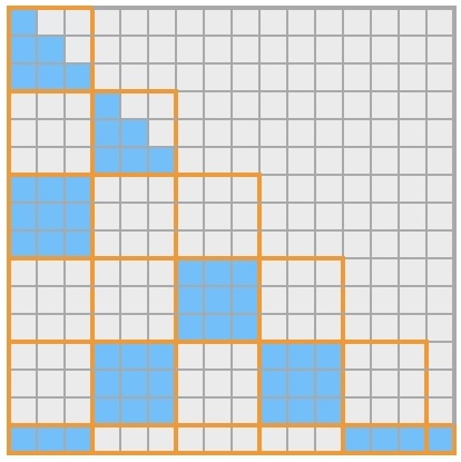
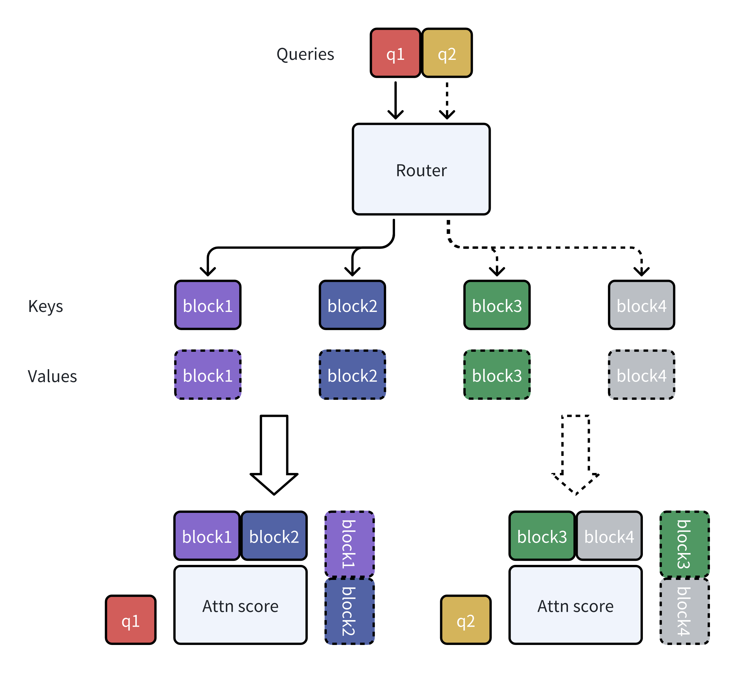
Block sparse attention partitions the sequence into blocks and selects only the most relevant blocks for each query, dramatically reducing computational complexity from $O(N^2)$ to $O(N \cdot k)$ where $k$ is the number of selected blocks. The left figure shows the the attention map of the block sparse attention, and the right figure shows Mixture of Block Attention (MoBA)'s workflow.

But this efficiency introduces a critical puzzle: how does the model know which blocks to pick? How can we be sure it isn't discarding the one crucial paragraph it needs from a sea of irrelevant text?

This post develops a simple statistical model to answer that question. I'll show that the success of block sparse attention isn't magic; it relies on a learned "similarity gap" that creates a strong enough signal to reliably pinpoint relevant information amid statistical noise.

An Abstract Model of Block Sparse Attention

To build intuition, I'll construct a simplified model. Let's assume for any given query $\mathbf{q}_j$, its goal is to find its one corresponding key $\mathbf{k}^*$ (the "signal"), while all other keys are treated as uniform "noise." This simplification helps isolate the core mechanism at play.

Assume $N$ input tokens with embeddings $\{\mathbf{x}_1, \mathbf{x}_2, \ldots, \mathbf{x}_N\} \subset \mathbb{R}^{d_{head}}$. These are projected into queries and keys:

Queries: $\mathbf{q}_i = \mathbf{x}_i W_Q \in \mathbb{R}^d$
Keys: $\mathbf{k}_i = \mathbf{x}_i W_K \in \mathbb{R}^d$

The $N$ keys are partitioned into $M$ non-overlapping blocks of size $B$ ($N = M \times B$). Each block is summarized by its centroid:

\mathbf{c}_i^K = \frac{1}{B} \sum_{\mathbf{u} \in K_i} \mathbf{u} \quad \text{for } i = 1, 2, \ldots, M

A query $\mathbf{q}_j$ must find the "signal block" containing its corresponding key $\mathbf{k}^*$. The query computes similarity scores with all centroids:

s_i = \mathbf{q}_j^T \mathbf{c}_i^K \quad \text{for } i = 1, 2, \ldots, M

Success is defined as the signal block $j^*$ (containing $\mathbf{k}^*$) achieving a rank within the top $k$ sampled blocks:

\text{Success} \iff \text{rank}(s_{j^*}) \leq k

Our goal is to understand the probability of this event.

The Key Mechanism: A Learned Similarity Gap

The signal block's score is:

s_{j^*} = \mathbf{q}_j^T \mathbf{c}_{j^*}^K = \frac{1}{B} \sum_{\mathbf{u} \in K_{j^*}} \mathbf{q}_j^T \mathbf{u} = \frac{1}{B} \left( \underbrace{\mathbf{q}_j^T \mathbf{k}^*}_{\text{signal}} + \sum_{\substack{\mathbf{u} \in K_{j^*} \\ \mathbf{u} \neq \mathbf{k}^*}} \mathbf{q}_j^T \mathbf{u} \right)

A well-trained model learns to maximize the similarity between a query and its corresponding key relative to irrelevant keys. We model this with two parameters:

Signal Similarity: $\mathbb{E}[\mathbf{q}_j^T \mathbf{k}^*] = \mu_{signal}$
Noise Similarity: $\mathbb{E}[\mathbf{q}_j^T \mathbf{k}_l] = \mu_{noise}$ for any irrelevant key $\mathbf{k}_l$

The similarity gap is defined as $\Delta\mu = \mu_{signal} - \mu_{noise} > 0$.

The expected score for the signal block mixes one signal term with $(B-1)$ noise terms, while any noise block $k$ has $B$ noise terms:

\mathbb{E}[s_{j^*}] = \frac{1}{B}(\mu_{signal} + (B-1)\mu_{noise})$$ $$\mathbb{E}[s_k] = \mu_{noise}

The signal block's expected advantage is:

\mathbb{E}[s_{j^*}] - \mathbb{E}[s_k] = \frac{\Delta\mu}{B}

This "learned similarity gap" is the mechanism that enables reliable block retrieval. But is this gap large enough to overcome random statistical fluctuations?

A Signal-to-Noise Ratio Analysis

To compute the probability of success, we must account for variance. We analyze the difference $D = s_{j^*} - s_k$ between the signal block and a specific noise block.

Modeling Assumptions

For a fixed query $\mathbf{q}_j$:

Dot products $\mathbf{q}_j^T \mathbf{u}$ are independent for all keys $\mathbf{u}$
Irrelevant keys: $\mathbf{q}_j^T \mathbf{u} \sim (\mu_{noise}, \sigma^2)$
Signal key: $\mathbf{q}_j^T \mathbf{k}^* \sim (\mu_{signal}, \sigma^2)$
In high dimensions with normalized vectors, $\sigma^2 \approx 1/d$

Deriving the SNR

The scores $s_{j^*}$ and $s_k$ are sums of these variables. By the Central Limit Theorem, they are approximately normal. We compute:

\mathbb{E}[D] = \mathbb{E}[s_{j^*} - s_k] = \frac{\Delta\mu}{B}

For the variance, since all dot products are independent:

\text{Var}(s_{j^*}) = \frac{1}{B^2}(\sigma^2 + (B-1)\sigma^2) = \frac{\sigma^2}{B}$$ $$\text{Var}(s_k) = \frac{1}{B^2}(B\sigma^2) = \frac{\sigma^2}{B}$$ $$\text{Var}(D) = \text{Var}(s_{j^*}) + \text{Var}(s_k) = \frac{2\sigma^2}{B}

Thus, $D \sim \mathcal{N}\left(\frac{\Delta\mu}{B}, \frac{2\sigma^2}{B}\right)$.

The probability that a specific noise block scores higher than the signal block is:

p = P(s_k > s_{j^*}) = P(D < 0)=\Phi\left( \frac{0 - \frac{\Delta\mu}{B}}{\sqrt{\frac{2\sigma^2}{B}}} \right)=\Phi\left( -\frac{\Delta\mu}{\sigma\sqrt{2B}} \right)

Substituting $\sigma^2 = 1/d$, we get:

p = 1 - \Phi\left( \Delta\mu \sqrt{\frac{d}{2B}} \right)

The key term is the Signal-to-Noise Ratio:

$$\text{SNR} = \Delta\mu \sqrt{\frac{d}{2B}}$$

A higher SNR means a lower probability $p$ of a single noise block being mis-ordered. For the signal block to be in the top-$k$ blocks, at most $k-1$ noise blocks can outrank it. The number of noise blocks that outrank the signal follows a binomial distribution with $M-1$ trials and success probability $p$:

P(\text{Top-}k) = P(\text{Binomial}(M-1, p) \leq k-1) = \sum_{i=0}^{k-1} \binom{M-1}{i} p^i (1-p)^{M-1-i}

For large $M$ and small $p$, this is well-approximated by a Poisson distribution with parameter $\lambda = (M-1)p \approx Mp$.

Statistical foundations. Top-left: How SNR affects the probability of misranking. Top-right: Distribution of outranking noise blocks. Bottom: Success probability curves and the effect of block size on SNR.

Practical Implications and Design Principles

The performance of block sparse attention is governed by the SNR. This leads to concrete design guidelines.

1. The Core SNR Ratio

The SNR = $\Delta\mu \sqrt{d/(2B)}$ shows that performance depends on:

Similarity Gap ($\Delta\mu$): A measure of training quality. Squared in the SNR's "power".
Architectural Ratio ($d/B$): Head dimension vs. block size.

To maintain performance when increasing $B$, one must increase $d$ or improve training to widen $\Delta\mu$.

2. The Power of the Similarity Gap

The similarity gap $\Delta\mu$ is the most powerful lever. Consider a model with $M=16$ blocks, $d=128$, $B=64$. Let's see how this plays out for different values of top-$k$:

Training Quality	$\Delta\mu$	SNR	$p$	$\lambda = Mp$	$P(\text{Top-2})$	$P(\text{Top-4})$
Poor	0.4	0.4	0.345	5.52	6.2%	31.5%
Good	0.8	0.8	0.212	3.39	21.5%	60.9%
Excellent	1.2	1.2	0.115	1.84	53.1%	89.1%

Doubling $\Delta\mu$ from 0.4 to 0.8 improves top-2 accuracy by 3.5× and top-4 accuracy by nearly 2×.

3. Architectural Trade-offs

Let's analyze a model with $M=16$, $\Delta\mu = 0.8$ ($\mu_{signal}=0.9$, $\mu_{noise}=0.1$).

Configuration	SNR	$p$	$\lambda = Mp$	$P(\text{Top-2})$	$P(\text{Top-4})$
$d=64$, $B=32$	0.8	0.212	3.39	21.5%	60.9%
$d=128$, $B=32$	1.13	0.129	2.06	47.0%	85.7%
$d=64$, $B=16$	1.13	0.129	2.06	47.0%	85.7%

Doubling $d$ or halving $B$ yields the same improvement: top-2 accuracy increases from 21.5% to 47%, demonstrating the $d/B$ trade-off.

4. The Long-Context Scaling Law

For very long sequences with many blocks $M$, the expected number of noise blocks that outrank the signal is $\lambda = Mp$. Using the Poisson approximation, the probability of being in the top-$k$ is:

P(\text{Top-}k) \approx \sum_{i=0}^{k-1} \frac{\lambda^i e^{-\lambda}}{i!}

For a desired success probability (e.g., 95%), we need $\lambda$ to be small relative to $k$. This gives us a useful design criterion: for reliable top-$k$ retrieval, we need $\lambda = Mp \ll k$.

Interactive Calculator: Experiment with different parameters to see how they affect the success probability of block sparse attention. Try adjusting the head dimension (d), block size (B), number of top blocks (k), and context length (L) to understand their relationships.

Let's see what this means for a million-token context ($N=2^{20}$) with $B=64$, giving $M=16,384$ blocks. We'll assume a good model with $\Delta\mu = 0.8$ and examine what's needed for different top-$k$ values.

Case 1: Top-8 retrieval with 95% success

We need $P(\text{Top-8}) \geq 0.95$, which requires $\lambda \approx 3.5$
This means $p = \lambda/M = 3.5/16384 \approx 2.14 \times 10^{-4}$
Required SNR: $\Delta\mu \sqrt{d/(2B)} = \Phi^{-1}(1-p) \approx 3.50$
Required dimension: $d = 2B \cdot (\text{SNR}/\Delta\mu)^2 = 128 \cdot (3.50/0.8)^2 \approx$ 2,450

Case 2: Top-32 retrieval with 95% success

We need $\lambda \approx 20$ for 95% success in top-32
This means $p = 20/16384 \approx 1.22 \times 10^{-3}$
Required SNR: $\approx 3.04$
Required dimension: $d \approx 128 \cdot (3.04/0.8)^2 \approx$ 1,850

This reveals a key insight: practical sparse attention systems that sample multiple blocks (e.g., top-32) can work with more reasonable head dimensions (in the low thousands) even for million-token contexts, whereas requiring top-1 accuracy would need impractically large dimensions.

An alternative is to increase the number of sampled blocks, $k$. For large $M$, the number of noise blocks that outrank the signal block, $Y$, follows a Poisson distribution with $\lambda \approx Mp$. To succeed with 95% probability, we need to sample $k \approx \lambda + 1.645\sqrt{\lambda} + 1$ blocks.

Consider a model with $d=128, B=64$ ($\implies$ SNR = 0.8, $p \approx 0.212$) and a context of $M=16,384$ blocks.
Expected mis-rankings: $\lambda = Mp \approx 16384 \cdot 0.212 \approx 3,473$
Required top-k: $k \approx 3473 + 1.645\sqrt{3473} + 1 \approx 3,571$
This means we must sample $k/M \approx 3571/16384 \approx \mathbf{21.8\%}$ of all blocks, significantly reducing the computational savings of sparse attention.

Required head dimension for 95% success rate at different context lengths. Notice how sampling more blocks (higher k) dramatically reduces the dimension requirements.

Conclusion

Block sparse attention is more than just a computational shortcut; it's a method that relies on the model's ability to learn clean, discriminative representations. Its success hinges on a single principle: the similarity gap ($\Delta\mu$) must be large enough to overcome the noise introduced by averaging keys into blocks.

Our analysis shows this relationship is governed by the SNR, $\Delta\mu \sqrt{d/(2B)}$, which provides a direct link between training quality ($\Delta\mu$) and architectural design ($d, B$). As we push towards million-token contexts and beyond, this framework reveals the true bottleneck: not just compute, but the fundamental challenge of learning representations with a nearly perfect signal-to-noise ratio.

Limitations

Our analysis makes several simplifying assumptions that merit discussion:

Single-Signal Simplification: We model each query as having exactly one relevant key, treating all others as uniform noise. In reality, queries aggregate information from multiple semantically related tokens.
Independence Assumption: We assume dot products between a query and different keys are statistically independent. In practice, keys within a block (e.g., consecutive words) are correlated. This likely reduces the effective variance of the block centroid, making selection easier than our model predicts. Therefore, our derived requirements for d should be seen as a conservative upper bound.
Fixed Parameters: We treat $\Delta\mu$ as a constant, though it varies across layers, heads, and semantic relationships in real models.

These simplifications mean our specific numerical predictions (like $d \approx 2,450$ for million-token contexts) should be taken as upper bounds rather than precise requirements. The actual dynamics involve semantic structure and correlations that work in favor of sparse attention.

Despite these limitations, the core insight remains: block sparse attention's effectiveness fundamentally depends on learning representations where the similarity gap between relevant and irrelevant content survives the averaging process.

References

BigBird: Transformers for Longer Sequences. Manzil Zaheer, Guru Guruganesh, Avinava Dubey, Joshua Ainslie, Chris Alberti, Santiago Ontanon, Philip Pham, Anirudh Ravula, Qifan Wang, Li Yang, Amr Ahmed. Neural Information Processing Systems (NeurIPS), 2020. arXiv:2007.14062
XAttention: Block Sparse Attention with Antidiagonal Scoring. Ruyi Xu, Guangxuan Xiao, Haofeng Huang, Junxian Guo, Song Han. Proceedings of the 42nd International Conference on Machine Learning (ICML), 2025. arXiv:2503.16428
SeerAttention: Learning Intrinsic Sparse Attention in Your LLMs. Yizhao Gao, Zhichen Zeng, Dayou Du, Shijie Cao, Peiyuan Zhou, Jiaxing Qi, Junjie Lai, Hayden Kwok-Hay So, Ting Cao, Fan Yang, Mao Yang. arXiv preprint, 2024. arXiv:2410.13276
MoBA: Mixture of Block Attention for Long-Context LLMs. Enzhe Lu, Zhejun Jiang, Jingyuan Liu, Yulun Du, Tao Jiang, Chao Hong, Shaowei Liu, Weiran He, Enming Yuan, Yuzhi Wang, Zhiqi Huang, Huan Yuan, Suting Xu, Xinran Xu, Guokun Lai, Yanru Chen, Huabin Zheng, Junjie Yan, Jianlin Su, Yuxin Wu, Neo Y. Zhang, Zhilin Yang, Xinyu Zhou, Mingxing Zhang, Jiezhong Qiu. arXiv preprint, 2025. arXiv:2502.13189
Native Sparse Attention: Hardware-Aligned and Natively Trainable Sparse Attention. Jingyang Yuan, Huazuo Gao, Damai Dai, Junyu Luo, Liang Zhao, Zhengyan Zhang, Zhenda Xie, Y. X. Wei, Lean Wang, Zhiping Xiao, Yuqing Wang, Chong Ruan, Ming Zhang, Wenfeng Liang, Wangding Zeng. EMNLP, 2025. arXiv:2502.11089

Citation

If you find this analysis useful and want to cite it in your work, you can use the following BibTeX entry:

@misc{xiao2025statistics,
  title={Statistics behind Block Sparse Attention},
  author={Guangxuan Xiao},
  year={2025},
  howpublished={\url{https://guangxuanx.com/blog/block-sparse-attn-stats.html}}
}

Configuration	SNR	\(p\)	\(\lambda = Mp\)	\(P(\text{Top-2})\)	\(P(\text{Top-4})\)
\(d=64\), \(B=32\)	0.8	0.212	3.39	21.5%	60.9%
\(d=128\), \(B=32\)	1.13	0.129	2.06	47.0%	85.7%
\(d=64\), \(B=16\)	1.13	0.129	2.06	47.0%	85.7%